

How To Add X And Y Into R Studio
Approximate fourth dimension: 60 minutes
Learning Objectives
- Plot graphs using the external package "ggplot2".
- Use the "map" function for iterative tasks on information structures.
- Consign plots for utilise outside of the R environment.
Setting up a information frame for visualization
In this lesson we desire to make plots to evaluate the average expression in each sample and its relationship with the age of the mouse. So, to this end, nosotros will be adding a couple of additional columns of information to the metadata data frame that nosotros can use for plotting.
Computing average expression
Let'due south take a closer look at our counts data. Each column represents a sample in our experiment, and each sample has ~38K values corresponding to the expression of different transcripts. We want to compute the average value of expression for each sample eventually. Taking this one pace at a time, what would we do if we just wanted the average expression for Sample 1 (across all transcripts)? We can use the R base parcel provided function called mean():
mean ( rpkm_ordered $ sample1 ) That is great, if we only wanted the average from one of the samples (1 column in a information frame), just we demand to get this information from all 12 samples, and then all 12 columns. It would be ideal to get a vector of 12 values that we tin can add to the metadata data frame. What is the best style to practise this?
Programming languages typically have a way to allow the execution of a single line of lawmaking or several lines of lawmaking multiple times, or in a "loop". While "for loops" are available in R, at that place are other easier-to-use functions that can accomplish this - for example, the apply() family of functions and the map() family of functions.
The map() family is a bit more intuitive to use than use() and we will be using information technology today. Withal, if you are interested in learning more than nigh theemploy() family of functions we take materials available here.
To obtain mean values for all samples nosotros can use the map_dbl() function which generates a numeric vector.
library ( purrr ) # Load the purrr samplemeans <- map_dbl ( rpkm_ordered , hateful ) The
mapfamily of functionsThe
map()family unit of functions is available from thepurrrpackage, which is function of the tidyverse suite of packages. More detailed information is available in the R for Data Science book. This family unit includes several functions, each taking a vector as input and outputting a vector of a specified type. For example, we can use these functions to execute some task/part on every element in a vector, or every column in a dataframe, or every component of a list, and so on.
map()creates a list.map_lgl()creates a logical vector.map_int()creates an integer vector.map_dbl()creates a "double" or numeric vector.map_chr()creates a character vector.The syntax for the
map()family of functions is:## DO NOT RUN map ( object , function_to_apply )If you lot would like to practice with the
map()family of functions, we accept additional materials available.
Creating a new metadata object with additional information
Because the input was 12 columns of information the output of map_dbl() is a named vector of length 12.
# Named vectors have a name assigned to each element instead of just referring to them as indices ([1], [2] and and then on) samplemeans # Check length of the vector before calculation information technology to the data frame length ( samplemeans ) Since we take 12 rows in the data frame, we can add the 12 chemical element vector as a cavalcade to our metadata data frame using the data.frame() function.
Before we add the new cavalcade, let's create a vector with the ages of each of the mice in our data prepare.
# Create a numeric vector with ages. Annotation that there are 12 elements hither age_in_days <- c ( 40 , 32 , 38 , 35 , 41 , 32 , 34 , 26 , 28 , 28 , 30 , 32 ) Now, we are set to combine the metadata data frame with the 2 new vectors to create a new data frame with five columns
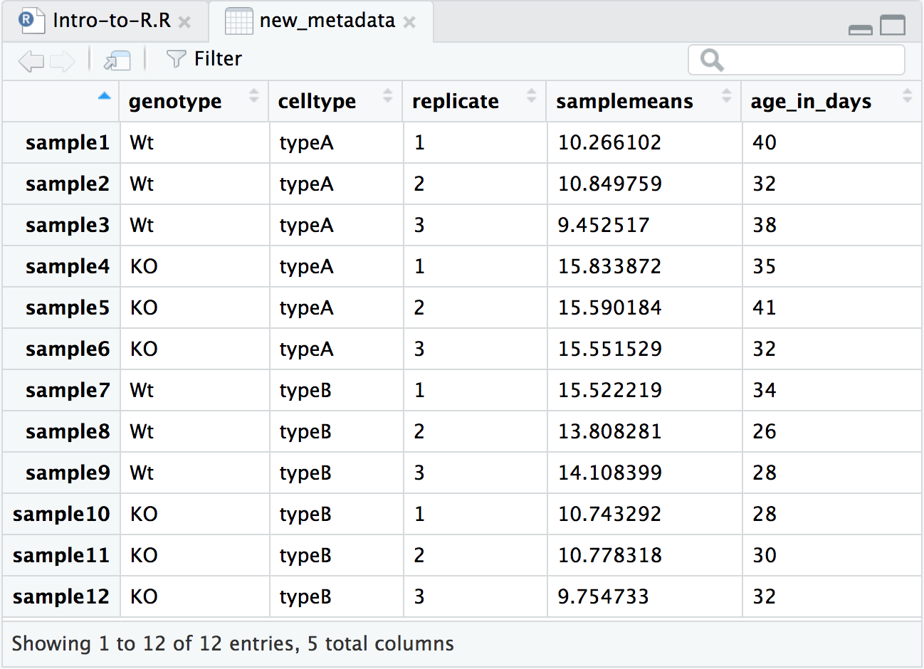
# Add the new vector as the final column to the new_metadata dataframe new_metadata <- data.frame ( metadata , samplemeans , age_in_days ) # Take a wait at the new_metadata object View ( new_metadata ) Nosotros are now set up for plotting and information visualization!
Data Visualization with ggplot2
When we are working with large sets of numbers it can be useful to display that information graphically to gain more insight. In this lesson we will be plotting with the popular Bioconductor package ggplot2.
If you are interested in learning about plotting with base of operations R functions, nosotros accept a short lesson available here.
The ggplot2 syntax takes some getting used to, but once y'all become information technology, you volition notice information technology'south extremely powerful and flexible. We will start with cartoon a elementary ten-y scatterplot of samplemeans versus age_in_days from the new_metadata data frame. Please note that ggplot2 expects a data frame every bit input.
Permit's start past loading the ggplot2 library:
The ggplot() function is used to initialize the bones graph construction, then we add to it. The basic thought is that you lot specify different parts of the plot using additional functions 1 afterwards the other and combine them into a "code chunk" using the + operator; the functions in the resulting code clamper are called layers.
Let's first:
ggplot ( new_metadata ) # what happens? You get an blank plot, because you need to specify boosted layers using the + operator.
The geom (geometric) object is the layer that specifies what kind of plot we want to draw. A plot must have at to the lowest degree one geom ; at that place is no upper limit. Examples include:
- points (
geom_point,geom_jitterfor scatter plots, dot plots, etc) - lines (
geom_line, for time series, trend lines, etc) - boxplot (
geom_boxplot, for, well, boxplots!)
Let'southward add a "geom" layer to our plot using the + operator, and since we want a scatter plot then nosotros will use geom_point().
ggplot ( new_metadata ) + geom_point () # notation what happens here Why do we go an error? Is the error message easy to decipher?
We go an error because each type of geom usually has a required set of aesthetics to exist set. "Aesthetics" are gear up with the aes() role and can be set either nested within geom_point() (applies merely to that layer) or within ggplot() (applies to the whole plot).
The aes() function has many different arguments, and all of those arguments take columns from the original data frame as input. It can be used to specify many plot elements including the following:
- position (i.e., on the x and y axes)
- color ("outside" colour)
- make full ("inside" color)
- shape (of points)
- linetype
- size
To start, we will specify x- and y-axis since geom_point requires the virtually basic information about a scatterplot, i.e. what you lot desire to plot on the x and y axes. All of the other plot elements mentioned above are optional.
ggplot ( new_metadata ) + geom_point ( aes ( x = age_in_days , y = samplemeans )) 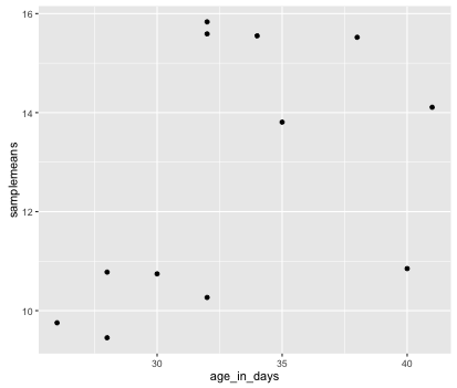
Now that nosotros have the required aesthetics, let'south add together some extras like colour to the plot. Nosotros tin color the points on the plot based on the genotype cavalcade within aes(). You lot will notice that there are a default fix of colors that volition be used and then we do not accept to specify. Annotation that the fable has been conveniently plotted for us.
ggplot ( new_metadata ) + geom_point ( aes ( 10 = age_in_days , y = samplemeans , color = genotype )) 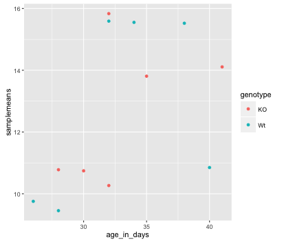
Let's attempt to have both celltype and genotype represented on the plot. To practise this we tin can assign the shape argument in aes() the celltype cavalcade, so that each celltype is plotted with a different shaped data signal.
ggplot ( new_metadata ) + geom_point ( aes ( x = age_in_days , y = samplemeans , color = genotype , shape = celltype )) 
The data points are quite pocket-size. Nosotros can conform the size of the information points within the geom_point() layer, but it should not be inside aes() since we are non mapping it to a column in the input data frame, instead we are just specifying a number.
ggplot ( new_metadata ) + geom_point ( aes ( x = age_in_days , y = samplemeans , colour = genotype , shape = celltype ), size = 2.25 ) 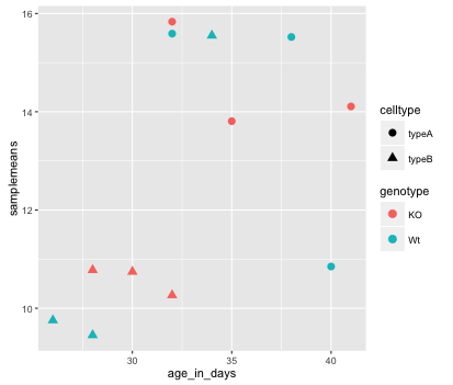
The labels on the x- and y-axis are also quite small and difficult to read. To change their size, we need to add an additional theme layer. The ggplot2 theme system handles non-data plot elements such as:
- Axis characterization aesthetics
- Plot background
- Facet label backround
- Legend appearance
There are congenital-in themes nosotros can use (i.eastward. theme_bw()) that more often than not change the groundwork/foreground colours, by calculation information technology as additional layer. Or we tin can adjust specific elements of the electric current default theme by adding the theme() layer and passing in arguments for the things we wish to change. Or nosotros can use both.
Let'south add a layer theme_bw(). Exercise the axis labels or the tick labels get any larger by irresolute themes?
ggplot ( new_metadata ) + geom_point ( aes ( x = age_in_days , y = samplemeans , color = genotype , shape = celltype ), size = 3.0 ) + theme_bw () Not in this case. Simply we can add arguments using theme() to change the size of axis labels ourselves. Since we are adding this layer on top (i.e later on in sequence), whatever features we alter will override what is ready in the theme_bw(). Here we'll increase the size of the axes titles to be one.v times the default size. When modifying the size of text we often use the rel() function. In this mode the size we specify is relative to the default. We can also provide the number vaue as nosotros did with the information point size, but tin be cumbersome if you don't know what the default font size is to begin with.
ggplot ( new_metadata ) + geom_point ( aes ( x = age_in_days , y = samplemeans , colour = genotype , shape = celltype ), size = 3.0 ) + theme_bw () + theme ( axis.championship = element_text ( size = rel ( 1.5 ))) 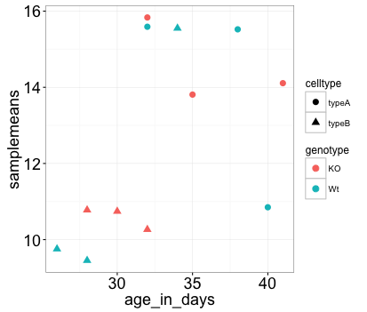
Notation: You can use the
example("geom_point")part hither to explore a multitude of different aesthetics and layers that tin be added to your plot. As you whorl through the unlike plots, take note of how the code is modified. Y'all tin utilize this with whatever of the different geometric object layers bachelor in ggplot2 to learn how you can easily modify your plots!
Note: RStudio provide this very useful cheatsheet for plotting using
ggplot2. Different example plots are provided and the associated lawmaking (i.eastward whichgeomorthemeto use in the advisable state of affairs.) We likewise encourage you to persuse through this useful online reference for working with ggplot2.
Do
- The electric current axis label text defaults to what we gave as input to
geom_point(i.e the cavalcade headers). We can alter this past adding additional layers chosenxlab()andylab()for the x- and y-centrality, respectively. Add these layers to the current plot such that the x-axis is labeled "Age (days)" and the y-centrality is labeled "Mean expression". - Use the
ggtitlelayer to add a title to your plot.
Note: Useful code to centre your title over your plot can exist done using theme(plot.title=element_text(hjust=0.v)).
Consistent formatting using custom functions
When publishing, it is helpful to ensure all plots have similar formatting. To practise this we can create a custom function with our preferences for the theme. Remember the construction of a role is:
name_of_function <- function ( arguments ) { statements or code that does something } Now, let's suppose nosotros always wanted our theme to include the following:
theme_bw () + theme ( centrality.title = element_text ( size = rel ( 1.5 )), plot.title = element_text ( size = rel ( 1.5 ), hjust = 0.five )) If there is nothing that nosotros want to alter when nosotros run this, then we do not demand to specify any arguments. Creating the function is simple; nosotros can just put the code inside the {}:
personal_theme <- function (){ theme_bw () + theme ( axis.title = element_text ( size = rel ( i.5 )), plot.title = element_text ( size = rel ( 1.5 ), hjust = 0.5 )) } At present to run our personal theme with any plot, we tin apply this function in place of the theme() lawmaking:
ggplot ( new_metadata ) + geom_point ( aes ( x = age_in_days , y = samplemeans , colour = genotype , shape = celltype ), size = rel ( 3.0 )) + xlab ( "Age (days)" ) + ylab ( "Hateful expression" ) + ggtitle ( "Expression with Age" ) + personal_theme () Boxplot
Now that we have all the required information for plotting with ggplot2, let's effort plotting a boxplot. A boxplot provides a graphical view of the distribution of information based on a 5 number summary. The top and bottom of the box represent the (i) first and (ii) third quartiles (25th and 75th percentiles, respectively). The line inside the box represents the (iii) median (50th percentile). The whiskers extending in a higher place and below the box represent the (iv) maximum, and (5) minimum of a data set up. The whiskers of the plot reach the minimum and maximum values that are non outliers.
Outliers are determined using the interquartile range (IQR), which is defined as: Q3 - Q1. Whatsoever values that exceeds i.5 x IQR below Q1 or in a higher place Q3 are considered outliers and are represented as points above or beneath the whiskers. These outliers are useful to identify any unexpected observations.
- Utilize the
geom_boxplot()layer to plot the differences in sample means between the Wt and KO genotypes. - Use the
fill upaesthetic to look at differences in sample means between the celltypes within each genotype. - Add a title to your plot.
- Add 'Genotype' as your x-axis label and 'Mean expression' equally your y-axis labels.
- Theme changes:
- Use the
theme_bw()office to make the background white. - Change the size of your axes labels to ane.5x larger than the default.
- Change the size of your plot title to one.5x larger than default.
- Heart the plot championship.
- Use the
Our final figure should look something like that provided below.
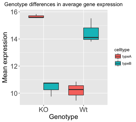
Code for making the boxplot above can exist found here
Note: If you lot wanted to modify the colors of these boxplots you would add some other layer
scale_fill_manual()to the code, and inside the function specify which colors you want to employ using thevaluesstatement. For example, if the gene cavalcade you are coloring with has 2 levels, you lot will need to give two values as followsscale_fill_manual(values=c("imperial","orange")).Annotation: You are not restricted to colors specified as above, yous have the choice of a lot of colors using their hexadecimal lawmaking, click here for more than data about color palettes in R.
Exporting figures to file
There are 2 means in which figures and plots tin be output to a file (rather than but displaying on screen).
(one) The first (and easiest) is to export directly from the RStudio 'Plots' console, past clicking on Export when the prototype is plotted. This volition give you the selection of png or pdf and selecting the directory to which you wish to save it to. It will also give you options to dictate the size and resolution of the output image.
(2) The 2d option is to employ R functions and accept the write to file hard-coded in to your script. This would allow you to run the script from beginning to stop and automate the process (non requiring man point-and-click actions to save). In R's terminology, output is directed to a particular output device and that dictates the output format that will be produced. A device must be created or "opened" in society to receive graphical output and, for devices that create a file on disk, the device must also be closed in order to consummate the output.
If we wanted to print our scatterplot to a pdf file format, we would need to initialize a plot using a role which specifies the graphical format you intend on creating i.e.pdf(), png(), tiff() etc. Inside the role you volition need to specify a proper noun for your image, and the with and tiptop (optional). This will open up the device that you wish to write to:
## Open device for writing pdf ( "figures/scatterplot.pdf" ) If you wish to modify the size and resolution of the paradigm you will need to add together in the appropriate parameters as arguments to the function when you initialize. Then nosotros plot the image to the device, using the ggplot scatterplot that nosotros but created.
## Make a plot which will be written to the open up device, in this case the temp file created by pdf()/png() ggplot ( new_metadata ) + geom_point ( aes ( x = age_in_days , y = samplemeans , color = genotype , shape = celltype ), size = rel ( three.0 )) Finally, close the "device", or file, using the dev.off() part. At that place are also bmp, tiff, and jpeg functions, though the jpeg role has proven less stable than the others.
## Closing the device is essential to salve the temporary file created past pdf()/png() dev.off () Notation one: You will non exist able to open and look at your file using standard methods (Adobe Acrobat or Preview etc.) until you execute the dev.off() function.
Notation 2: In the case of pdf(), if you had made boosted plots earlier closing the device, they will all be stored in the same file with each plot normally getting its own page, unless otherwise specified.
This lesson has been adult by members of the didactics team at the Harvard Chan Bioinformatics Core (HBC). These are open access materials distributed under the terms of the Creative Eatables Attribution license (CC BY four.0), which permits unrestricted use, distribution, and reproduction in whatever medium, provided the original author and source are credited.

How To Add X And Y Into R Studio,
Source: https://hbctraining.github.io/Intro-to-R/lessons/07_ggplot2.html
Posted by: kelleyandon1984.blogspot.com
0 Response to "How To Add X And Y Into R Studio"
Post a Comment